Into view: hiking and cycling through the Kaiserwinkl

After mapping shared travel destinations, I came back to Kössen for the next #30DayMapChallenge experiment. This time I wanted to answer a more local question: what comes into view as you move through the mountains?

A route line tells me where a path goes. An elevation profile tells me roughly how much climbing to expect. Neither tells me whether a ridge blocks the view of the mountains behind it, or when that view might open up.

A viewshed gets closer to that question. It uses an observer position and an elevation model to work out which terrain has an unobstructed line of sight from that point. Rather than calculating one view from a lookout, I wanted to follow how it changes along a route.

Follow the route, watch the view change

Open the figure separately · View a static map

Two routes from the same village square

I started with a hiking route from Kössen Dorf to Taubenseehütte. The first version kept too much empty space around the path. Moving the hike into the upper-right corner and extending the terrain south and west made a more useful composition: the path stays visible, but there’s room to see what happens towards Wilder Kaiser.

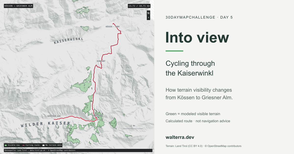
For the cycling route, I chose a path south through Schwendt and Griesenau, then west into Kaiserbachtal to Griesner Alm. The similar names are worth untangling: Griesenau is at the valley entrance, while Griesner Alm is farther inside it. I gave this view a closer frame around the route.

I used the same mapped starting point in Kössen for both. The routes follow connected OpenStreetMap networks rather than straight lines between endpoints. Neither is a Strava activity or a GPS recording of a trip I took.

Route	Calculated length	Visibility samples	Approximate spacing
Kössen → Taubenseehütte	4.88 km	99	50 m
Kössen → Griesner Alm	18.71 km	126	150 m

I made the cycling calculation prefer quieter roads where the network permits it, but that doesn’t produce a continuous traffic-free cycle path. Parts still use roads with motor traffic. One Kaiserbachtal segment also has incomplete bicycle-access tagging. I kept the single reviewed exception and the tourism-board description used to assess it in the cycling method, rather than leaving that routing decision undocumented.

I used the large curved Kaiserwinkl label for the region around Kössen, Walchsee, Schwendt and Rettenschöss. It’s there to give the map some regional context, not to mark a summit or draw an administrative boundary. The smaller place names and red route do the locating.

Terrain rather than a panoramic photograph

I started with Land Tirol’s laser-derived 5 m digital terrain model, sampled the extraction at roughly 10 m and reprojected it onto a 20 m grid for this prototype. The source resolution and the analysis resolution aren’t the same thing. Calling the result a 5 m analysis would overstate what I actually calculated.

For each sampled route position, I placed the observer 1.7 m above the ground. The preparation script scans 16,384 directions, checking terrain every 10 m along each ray, up to 32 km away. As it moves outward, it keeps track of terrain that blocks lower ground behind it. That maximum distance is only a limit on the calculation: the elevation extract and its missing-data areas can stop it sooner.

Two choices matter when reading the green areas:

• This is bare-earth terrain. Trees and buildings don’t block the view, even where they would in real life.
• Missing terrain ends a ray. It is not silently filled with flat ground. German terrain is absent from this extract, and those gaps are hatched.

I also left out Earth curvature, refraction and weather, so distant visibility is approximate, particularly towards larger mountains. I haven’t checked the results against a field survey or an independent reference GIS calculation. This is what the terrain model predicts, not a guarantee of what you’d see on the walk or ride.

Calculate once, animate the result

I used Three.js to render the map, but kept the visibility calculation out of the browser. Repeating a GIS analysis on every animation frame would be unnecessary when the terrain and route samples are already fixed.

Instead, I calculate each viewshed during preparation and save it as a single-channel mask. The browser moves the observer along the actual route vertices and swaps in the nearest visibility sample. That lets the marker move continuously while visibility changes in discrete steps. I didn’t interpolate visibility between samples or blur the edges into an extra visible area.

I gave each route 30 seconds of playback at a constant distance-based speed. That’s enough to follow the changing view without pretending to estimate how long the hike or ride would take. The camera stays fixed while the marker moves.

Loading the masks turned out to need another pass. The initial code decoded large grayscale PNG sheets into RGBA images, read them back through a canvas and copied one channel out again. The downloads were small, but the temporary pixel buffers weren’t. I was making the browser expand the data just to throw most of it away.

I switched to gzip-compressed single-channel buffers and the browser’s native decompression stream, loading two pages concurrently to keep memory use down. PNGs remain as a compatibility fallback. In one local Chromium comparison, startup went from about 838 ms to 152 ms. I wouldn’t generalize that timing to every browser, but it helped confirm where the time was going: pixel conversion rather than network transfer.

Separate the terrain from its colours

I kept the terrain relief and visibility masks as grayscale assets and applied their colours at runtime. That meant I could adjust the design without recalculating all the viewsheds.

That separation was useful while working on the visual hierarchy. A dark basemap made the map feel heavier than the previous challenge entries. Flattening it too far lost the very mountain structure the viewshed was meant to explain. I ended up keeping the directional slope shading while giving the land a lighter gray tone.

I took the light-gray land and leafy-green highlight from a map reference, with a darker green boundary on the inside of the visible area. Green means visible terrain here, not forest or land cover. I kept the route red with a white casing and placed the moving marker above the fill. The route, visibility mask and numbered photo stops also have different shapes, so reading them doesn’t depend only on distinguishing red from green.

The curved labels use the same monospace family as the smaller labels, with more spacing and a pale halo. They sit above the tint so the animation doesn’t wash them out, but below the route and settlement labels. It’s the kind of hierarchy Datawrapper describes in its colour guidance: context should support the important information, not compete with it. The particular colours are a design choice, not an official hiking palette.

Photographs as context, not validation

I added numbered photo stops to connect the terrain model to recognizable places. Selecting one pauses playback, jumps to its route-distance anchor and updates the photograph card. I put the same buttons on the elevation profile too, so finding a badge on the map isn’t the only way to reach a stop.

This version has four photo stops on the hike and ten on the ride, with the same Kössen photograph at the start of both. I supplied some of the upper hiking photographs; the other images come from Wikimedia Commons.

The photos come from different dates and seasons, not one continuous trip. I matched their camera positions approximately to the nearest route segment, although some were taken away from the calculated track. I kept the dates, camera offsets and credits visible to make that clear. A nearby photo isn’t a validation of the viewshed, and the model doesn’t know which way the camera was pointing.

The Commons images are CC BY-SA 4.0, with individual authors and source links. I kept my supplied photographs separately marked used with permission rather than giving them a Creative Commons label. The photo notes record which terms apply to each.

Sources and a pinned copy

As with the previous entries, I stored a local snapshot with the post. Opening it doesn’t fetch live terrain tiles, routing responses or remote libraries. I also made the route selector load one visualization at a time, rather than keeping two large WebGL scenes running together.

• Terrain and derived visibility: Datenquelle: Land Tirol - data.tirol.gv.at, CC BY 4.0 with the published terms and extensions.
• Routes and selected network metadata: © OpenStreetMap contributors, ODbL 1.0.
• Photographs: individual Commons credits and CC BY-SA notices, plus separately permitted owner images. See the photo notes above.
• Renderer: locally bundled Three.js 0.170.0, MIT. The interface uses plain HTML, CSS and JavaScript.

Downloads: hiking route, cycling route, hiking method, cycling method and snapshot manifest. The challenge repository contains the preparation scripts.

For a later animation export, renderAt(timeSeconds) can drive the same scene used for interactive playback. For now, I’ve included the interactive map and a static preview, not a rendered GIF.

What interests me most is the change along the way. A lookout point asks “what can I see from here?” Following a route turns it into “when does that view appear, and when does the terrain take it away?”

I used Pi Coding Agent with gpt-6.1-sol for source inspection, data preparation, implementation, writing assistance and checks.

Three.js is probably more machinery than this version needs. It handles the texture compositing and shaders well, but a fixed, top-down map with precomputed visibility could also work with a lighter Canvas renderer. I started with different ideas in mind that would have made fuller use of Three.js. As the scope changed, I kept the stack rather than rewriting a working renderer. It’s a consequence of how the experiment developed, not a requirement for making this kind of map.

---