Shared destinations

For Day 4 of the #30DayMapChallenge, the theme is Clusters.

After outlining ski resorts, I wanted to look at travel from the other direction: where do people from a particular country stay?

I ended up with a map where each city attracts a small cloud of bubbles. Each bubble represents the overnight stays of residents from one country in that destination. Selecting a country brings its bubbles forward while leaving the others visible for context.

One country, many destinations

Download the adapted CSV · Watch the animated country tour

Finding country-to-city data

Finding suitable data was the first hurdle. Country-to-country tourism statistics are easier to find than a consistent European city breakdown. I looked at Eurostat’s selected-city accommodation data, but the table I checked separates domestic and foreign guests rather than individual residence countries. Useful for other questions, but not for following visitors from the Netherlands across cities.

I used TourMIS, which brings together tourism statistics contributed by destinations. Its ECM-J8 report provides a matrix of origin markets and cities. The extract used here covers 2024, downloaded on 4 November 2026, with each destination’s preferred bednight definition.

The source matrix has 154 reporting destinations. I removed aggregate markets such as continents, foreign/domestic totals and residual “Other” groups. Keeping those alongside individual countries would count the same activity twice. That left 5,321 reported individual-country–destination pairs, spanning 61 origin countries.

I framed the map around Madeira, Trondheim and Rēzekne, which puts 147 destinations inside the geographic selection. Those account for 5,205 reported pairs, or 5,060 with domestic stays excluded. I kept destinations outside the frame in the downloadable data too.

One detail worth keeping in mind: “visitors from the Netherlands” means people resident there, not necessarily Dutch nationals. I don’t have their home cities, departure points or itineraries.

Let the city pull its bubbles together

The starting point was D3’s Clustered Bubbles. In that example, group attraction and collision forces pull related circles into clusters while keeping them apart.

I replaced the example’s group attractors with the destinations’ projected geographic positions. Every reported origin-country bubble for Vienna gets pulled towards Vienna; every bubble for Paris towards Paris. A collision force makes room for neighbouring circles. I kept colour out of the grouping: only the selected source country gets the accent colour, rather than assigning colours to destinations or suggesting different types of tourist.

So these are geographic bubble clusters, not tourism segments discovered by a clustering algorithm. The point is to separate overlapping records while keeping each destination’s different origins together.

Making that room means moving bubbles away from their cities. The tiny dark dots mark the destination anchors. I added a short line back to the anchor when you inspect a bubble, so you can see where it belongs. The ranked destination buttons offer the same interaction from the keyboard. The scattered circles aren’t extra cities or individual accommodation locations.

I used one fixed area scale for person-nights across both filter modes. The largest bubble represents 20,255,819 person-nights. At the small end, counts below about 38,036, including reported zeros, get a minimum marker size so they’re still possible to inspect. Those tiny circles aren’t strictly area-proportional, and zero counts don’t get connection lines.

Simulate once, then load the result

The initial version ran the force layout in the browser. It worked, but waiting for thousands of circles to settle didn’t add anything when the data and destination coordinates hadn’t changed. There was no reason to make each visitor repeat the same calculation.

I also ran into a filtering mistake. Hiding domestic bubbles left their collision space behind, producing a map full of circular holes. Removing a record from the display wasn’t enough; it had to be left out of the simulation too.

I moved the simulation into the preparation step and saved two independent layouts: one with domestic stays and one without. Each uses only the records it will display. The domestic filter removes every matching origin–destination country pair, not just those belonging to the selected origin. The browser loads the saved coordinates as ordinary local data, so changing the filter can switch compositions immediately.

Selecting another source country changes highlighting, connections and the ranking—not bubble positions. Resizing scales the composition uniformly instead of starting another simulation. That keeps the geography and collision spacing aligned without stretching the circles.

The projection fit needed attention too. Fitting around the occupied destination footprint, rather than the empty corners of a geographic rectangle, brought the view about 28% closer without dropping any included destinations. I used a Lambert azimuthal equal-area projection centred at 10°E, 49°N to avoid Mercator’s northern area exaggeration. This is D3’s spherical implementation, not an exact EPSG:3035 transformation.

Bundling the connections

Highlighting bubbles shows where a country’s stays appear. Lines make that relationship easier to follow, but drawing a separate straight spoke to every destination quickly gets busy.

I used the principle behind hierarchical edge bundling: nearby relationships share intermediate control points before branching towards their endpoints. Here, the hierarchy is constructed geographically, not taken from a transport network.

In the preparation script, I first separate targets into eight direction sectors from the source, then recursively split them into spatial groups. That produces chains of control points which D3’s existing bundle curve can render. I didn’t need another bundling library or a force simulation in the browser. Each domestic-filter mode gets its own saved connections.

The lines end at the actual city anchors, not at the displaced bubbles. Their widths are uniform; overlapping branches appear darker, but that darkness isn’t a calibrated volume scale.

The source end needed a different compromise. I have a residence country, but no departure city to put on the map. I used a labelled representative point for each country, usually a GeoNames capital or seat record, choosing the largest population when there are several candidates. That gives the lines somewhere to start without claiming everyone departed from that city.

When a source point falls outside the visible viewport, I leave it there and clip its lines at the edge. Only the directional country label moves to the edge. Calling the whole country “off-map” wouldn’t be accurate when part of it is visible, as with Turkey or Ukraine.

Getting the clipping right took another pass. The saved SVG composition and the visible viewport aren’t necessarily the same rectangle: uniform scaling can leave extra space beside or above the map. Clipping at the saved rectangle cut lines off before they reached the visible edge. I changed the renderer to update the clipping rectangle and edge labels for the actual viewport, while leaving the saved geometry alone.

The bundled lines make the relationships easier to follow, but they aren’t observed routes. Their shared branches don’t represent airports, roads, border crossings or places where travellers met. That’s a tempting reading of this kind of map, and one the data can’t support.

A tour without the controls

The animated GIF walks through all 61 source countries, alphabetically, at 1.2 seconds per country. A loop takes 73.2 seconds. Domestic stays are excluded and the bundled connections are enabled throughout.

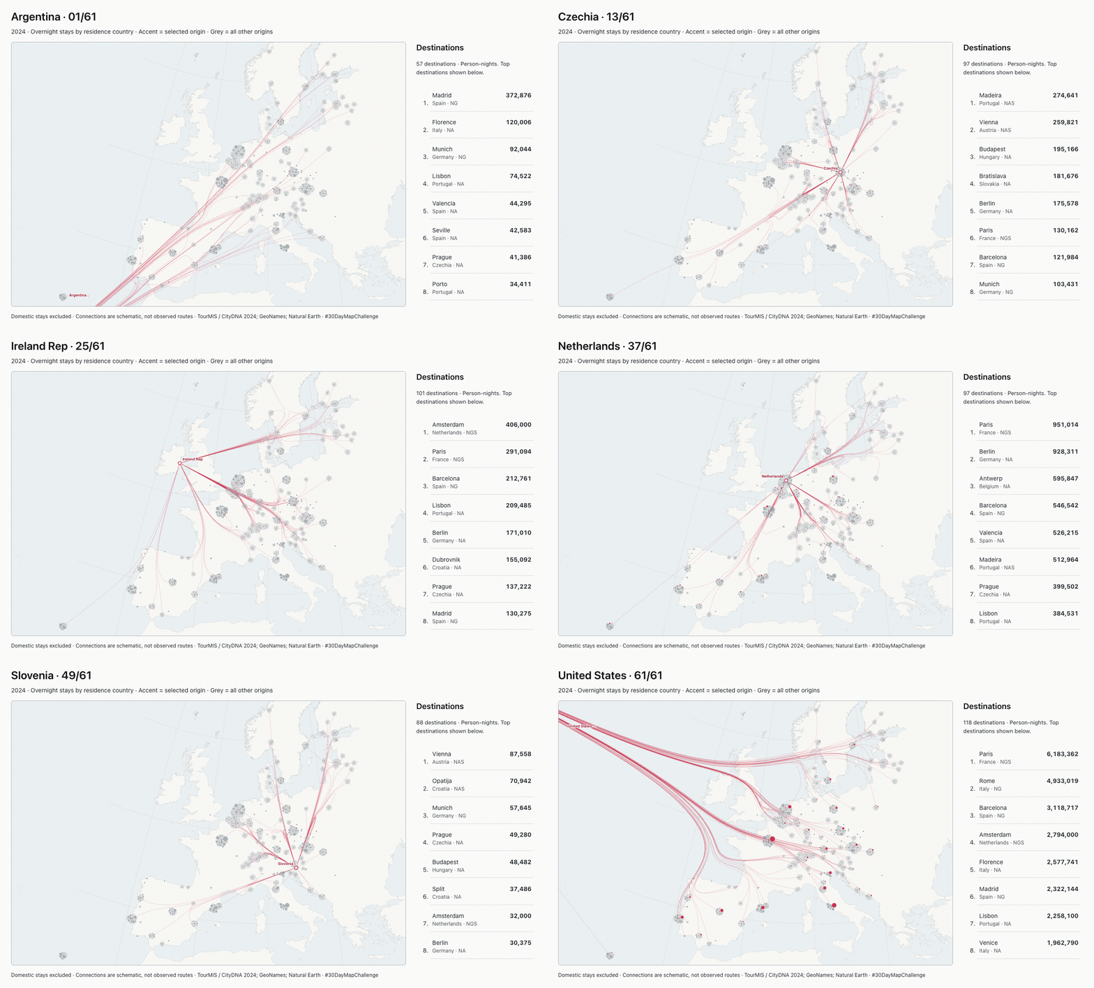
I reused the interactive map’s saved geometry for the export, with country names, progress, the selected-source ranking and attribution in each frame.

Sources, limitations and a pinned copy

The wide-figure and local-iframe setup from Day 3 came in useful again. I stored a snapshot of the map, data and animation with this post, so later edits to the challenge site won’t silently change what you see here. The same-origin bridge handles theme and iframe height. On desktop, the map and ranking share a fixed-height panel; on narrower screens, they stack.

• Tourism counts: TourMIS / CityDNA, ECM-J8, annual 2024, © MU Vienna and contributing statistical providers. The published reuse terms permit accurate reproduction and adaptation with source attribution and an extraction/adaptation notice. This is an adapted extract under custom terms, not a claim of a standard open-data licence.
• Destination and representative source points: GeoNames, CC BY 4.0. Madeira uses Funchal and Haarlemmermeer uses Hoofddorp as representative points.
• Land: Natural Earth, public domain.
• Rendering: local D3 v4.13.0, BSD-3-Clause. No visitor-time tourism API, tile service or remote library is needed.

The source definitions remain a limitation. Some destinations report hotels, others broader paid accommodation; some cover the city, others the greater-city area. Reporting areas can overlap too. I wouldn’t add these counts up into a European travel total. Those differences matter more than an extra digit in the ranking.

The useful result for me is being able to follow one country’s reported destinations without hiding everyone else. Most of the work went into making that readable without implying more than the data says. The counts are reported observations; the displaced bubbles, shared branches and representative country points are choices I made to draw them. Keeping that distinction visible matters more than making the lines look like a detailed account of actual journeys.

I used Pi Coding Agent with gpt-6.1-sol for data inspection, preparation, implementation, export and checks.

---